In this session we will introduce the ingredients we need to perform a molecular dynamics simulation. It is a mesh up of information you can find scattered on different sources. 1
Getting ready
For this tutorial, download the following source file. You should know how to untar, but let’s remind it:
$ tar xvzf tutorial2.tar.gz
There should be two folders: alanine-dip/ and bpti/.
Overview
Let’s recap the so called MD machinery.
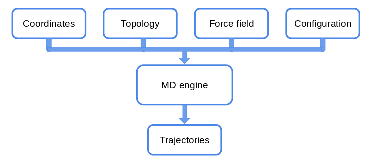
In today’s tutorial, we will focus on the files that contain the information on the system we want to study.
May the Force (field) be with you!
The idea is to solve the Newton’s equations of motion for all the atoms in the system. For each atom in 1D we can write:
\[m\frac{d^2 x}{dt^2} = -\nabla U\]We need then to know what the potential \(U\) is. The set of functions and parameters that composes the \(U\) is called Force Field (ff from now on).
The idea behind ffs is to mimic the experimental behaviour of proteins with a potential for atoms that has a feasible computational cost. There are several force fields available, such as:
- CHARMm, AMBER for all-atom simulations;
- Martini for coarse grained simulations.
Each ff has its own functional form and its protocol to define parameters. The parameters, in fact, hide under the hood assumptions that make the functional formation viable for simulations. Mixing CHARMm parameters with the AMBER potential, to mention two of the most popular ffs, will lead you to unreliable results.
Do not mix parameters from different force fields!
Moreover, ff parameters evolve as more data and simulations are gathered.
Check for the latest version of force fields!
We will mainly use CHARMm ff (version 36).
In general, each force field has two main parts (we are omitting the dependence on the coordinates and parameters that will be clear in the following): $$ U_{ff} = U_{bonded} + U_{non~bonded} $$
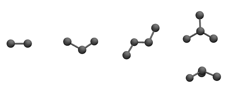
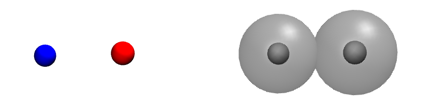
Let’s have a graphical representation.
Bonded interactions
Non-bonded interactions
As their name suggest, we can define interactions for covalently bonded atoms as:
\[\begin{align*} U_{bonded} & = \sum_{bonds} \frac{1}{2}k_{bond} (r_{ij} - r_0)^2 \\ & + \sum_{angles} \frac{1}{2} k_{angle} (\theta_{ijk} - \theta_{0})^2 \\ & + \sum_{dihedrals} k_{\phi,n} [\cos(n\phi_{ijkl} +\delta_n) +1]\\ & + \sum_{impropers} k_{improper} (\chi_{i^{*}jkl} - \chi_0)^2 \end{align*}\]but we have also to take into account non-bonded interactions between molecules and within molecules:
\[\begin{align*} U_{non~bonded} & = \sum_{nb~pairs} \Big[ \frac{q_i q_j}{4\pi\epsilon_0 r_{ij}} + \Big(\frac{A_{ij}}{r_{ij}^{12}} - \frac{B_{ij}}{r_{ij}^6}\Big)\Big]\\ \end{align*}\]Alanine dipeptide
Alanine dipeptide is a small peptide usually used to study protein backbone
dynamics. It consists of an ALA in the middle equipped with two minimal peptide bonds. The N terminus NH2 gains an acetyl group CH3CO, while the the C terminus
COOH obtains a methylamide CH3NH.
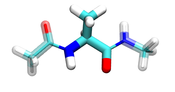
ACE - ALA - NME
How many carbon atoms are in the alanine dipeptide?
Are C atoms bonded with the same kind of atoms each time they appear?
A pdb and a top file for the alanine dipeptide is provided.
Let’s inspect the content of these files.
Use Vim! :)
In the same folder you have also a configuration file called vacuum.namd.
It is required to launch NAMD and perform the simulation. It is a Tcl
script were you can set the parameters of your simulation, the algorithms you want
to use, and the output.
Let’s open it as well.
Let’s run the simulation! It will take few minutes.
$ namd2 vacuum.namd > ala_vacuum.log &
What does > and & do?
Try to use the tail command:
$ tail -f *.log
Use ctrl-s to stop the shell screen if it is too fast. To resume the scroll,
use ctrl-q.
After the simulation is completed, load with the Tk console in VMD
the pdb and the trajectory.
% mol new dip.pdb
% mol addfile file.dcd waitfor all
Let’s compute the dihedral angles \(\phi\), whose definition is \(C_{i-1}-N_{i}-C\alpha_{i}-C_{i}\), and \(\psi\), dihedral defined by \(N_{i}-C\alpha_{i}-C_{i}-N_{i+1}\).
Hint: you measure,4, Extension.
Coordinates: PDB
We have already see a pdb file few moments ago.
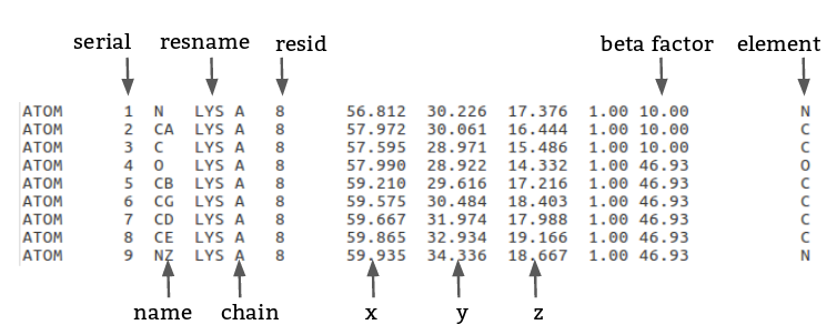 Let’s go the Protein Data Bank website and search for the
structure
4pti.
Let’s give a brief overview of these columns
-
serial: integer associated to each atom; -
name:atom nameof each atom (see figure below); -
resname: 3-letter code for protein, it can be a 4-letter code for fancy residues; -
chain: 1-letter identifier for each chain in a pdb; -
x,y, andz: try to guess; -
occupancy: usually1.00, it can be less than 1 if the structure is not univocally resolved; -
beta factor: temperature \(\beta_i = \frac{8\pi^2}{3}~msf_i\), it is related to the flexibility of the residue; -
element.
Regarding the atom names, they follow the star convention:
from \(\alpha\) (of the Carbon \(\alpha\)) to \(\beta, \gamma, \delta\)…
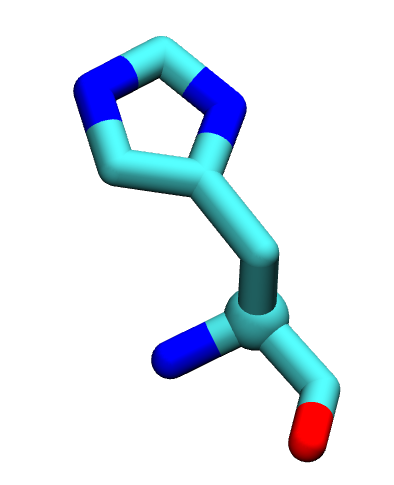
Histidine, as a constellation.
PDB files have a fixed format. Do not modify them manually if you are unsure of the outcome!
Move the pdb file from ~/Download/ into QCB_course/bpti/.
Let’s open it (with ViM!). For sake of safety, use:
$ vim -R 4pti.pdb
Let’s search the keyword we already know. Type in the Vim Normal mode:
/ATOMS (note the white space after the S).
ATOMS, HETATM define the rows in which atoms are written. The first is used
for the atoms of the proteins, ligands and water atoms are defined by the latter.
Let go at the beginning of the file (gg in ViM).
There are a lot of information, most of the are experimental data.
They are characterised by the keywords in the first column.
Some of them will be explained in the next lessons.
Now, go to the first SEQRES (search within ViM).
Let’s focus on the SSBOND keyword. In this section, if present, disulfide bonds
are defined.
These are bonds between the sulfur S atoms of two close cysteins.
Disulfide bonds play an important role in the folding and stability of some proteins,
therefore you have to include them in your future structure.
Write down the resid of the disulfide bonds.
Load the pdb with VMD, and remove the water from the visualisation. Visualise in Licorice, if present, aspartic acids, glutammic acid, lysine and arginine.
Visualise the disulfide bridges.
Does VMD create a link between 2 close sulfur atoms? Is it "real"?
Visualise the protein using Beta as Coloring method.
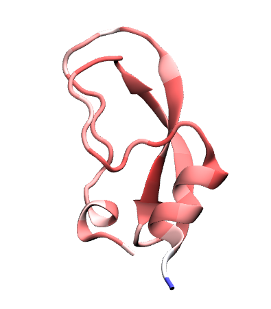
Does the colour scheme fit with your intuition?
Let’s write a new pdb without the water, since it will be useful for the psf file.
-
with
awk; -
within VMD:
% set prot [atomselect top "protein"]
% prot writepdb only_bpti.pdb
You should have (not) successfully create a new pdb file. Why?
NB: Usually the water molecules in a pdb can play an important role in the
protein biological function. In general, it is a good practice to keep them in
your final system.
Topology: .psf and .top in CHARMm
Let’s download the latest version of the CHARMm ff
and extract it into our QCB_course/ folder.
From now on, we will use topology for referring to the top_* files of the
force field, and structure for the psf file.
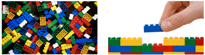
Topology file: a collection of bricks. PSF file: a subset of the top file arranged in a particular fashion.
The idea is to use the top file to construct the psf of our system.
First of all, let’s list all the file inside this folder. As you can see, the topology files are divided into categories: prot, lipid, na…
Open the top_all36_prot.rtf (again with ViM) in a read-only mode.
You will see a first part with the MASS definition, then the RESI keywords, and eventually the PRES keywords.
This top file is like a dictionary, with all the possible words (RESI) you can
use in your sentence (i.e. system).
The PRES are the so-called patches and they allow us to modify some residue if
you have a different protonation state, want to combine two residues, add a terminus…
PSF
The PSF file contains the information of your system structure and the charge
information.
Each segment of the system not covalently bound to others must have a separate
psf file. For a single-chain protein in solution is trivial. You have also to write
different psf if your system consists of several units, i.e. a multimer.
To write a psf file, we will use VMD with the Tk console.
You can write it as a script and load it in the tk console.
# load the namespace we need
package require psfgen
# read the information from the topology file
topology _correct_path_to_what_top_file_to_use?
# build the protein segment with name BPTI
segment BPTI {
pdb _yours_.pdb
#autoregenerate angles and dihedrals by default, NTER CTER
}
# Write down the patches we need to apply (What patches?)
patch _Patchname_ _segmentName_:_resid_ _segmentName_:resid
patch _Patchname_ _segmentName_:_resid_ _segmentName_:resid
patch _Patchname_ _segmentName_:_resid_ _segmentName_:resid
# using alias due to different atom name in pdb vs charmmff
pdbalias atom ILE CD1 CD
# readind the coordinates
coordpdb _yours_.pdb BPTI ;# write the segname!!!!!
# guess missing coordinates: are there missing atoms?
guesscoord
# write the structure and coordinate files
writepsf out.psf
writepdb out.pdb
If there are no errors, load first a new molecule with the psf and then the
pdb file.
Check the N-ter and C-ter with respect to the patches in the top file.
You can also use Extension -> Autopsf to generate the psf file, and most of the things will run behind the scene. ;)
To check whether the psf is ok, we can also run a small minimisation.
NAMD used an improved version of the conjugate gradient. The aim of the minimisation is two-fold:
- to remove the steric clashes that can be present when building a system adding elements;
- to move your structure into the ideal one provided by the topology file, with equilibrium distances, angles…
To launch the minimisation, use the minimise.namd that have to be completed and launch it with:
$ namd2 minimise.namd > bpti_min.log&
NB: with a single core it takes >30min for 1kk steps.
Load the trajectory and have fun.
Further Notes
- PSFGen user guide, already in your computer in the VMD installation folder (plugin subfolder).
Notes
-
No reference at the moment. ↩