In this session we will build the setup, analyse the configuration file and perform a small analysis of a system.1
I encourage you to have a look at the sources provided you at the end of the tutorial.
Getting ready
For this tutorial, download the following source files. You should know how to untar, but let’s remind it:
$ tar xvzf tutorial3.tar.gz
There should be four folders: bpti_trypsin/, common/, implicit/ and
explicit/.
Overview
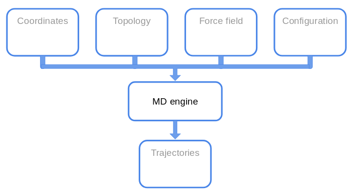
Let’s recap the so called MD machinery.
What files do we need?
PAR file
Last time we saw the several files, but we did not have a look at the parameters
file.
Let’s open par_all36m_prot.prm with ViM.
For each interaction we saw last time there should be a section in the
parameters file.
Do you see other potential functions not defined in the last lesson?
We mentioned that the force field has to be taken as a whole, since several approximations are hidden in the parameters definition.
Other parameters must be set for the non-bonded interactions (the exact meaning
will be defined in other lessons):

The meaning of these commands is not important for this tutorial, but the take-home message to remember is:
"You should **not** change parameters at your own will, unless you want to introduce a systematic error in your simulation and make them useless."
or, in another way:
First rule of the FF-Club is **Do not mess with the FF**.
 (Credits: La Scienza Coatta)
So, now we have an (almost) complete overview of the files we will deal with.
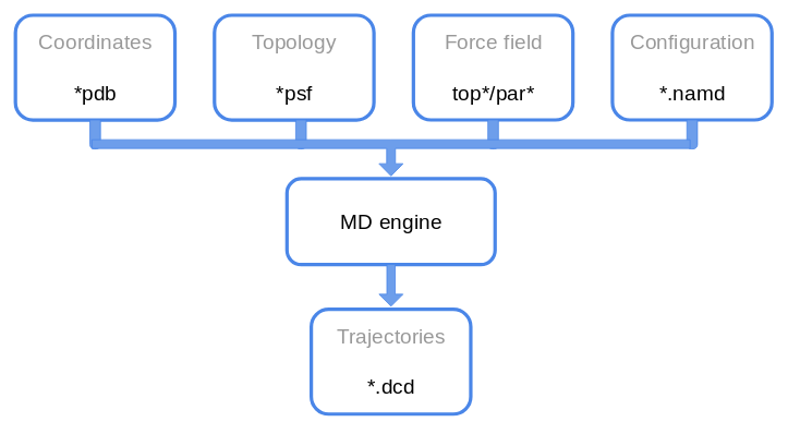 Congrats for the correct answer! ;)
The Problem
Before launching a simulation, let’s see what are the time scale we can investigate. For now, with MD we mean all-atom MD.
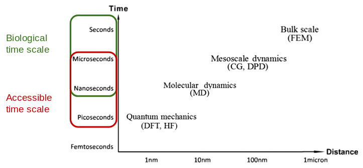
From the picture above we see that we are constrained both spatially and in the simulated time, since the idea is to publish and we don’t have infinite resources (someone pays the bill for the electric power used by computers).
When you decide to perform a simulation some questions should be answered in advance:
- What process do I want to investigate? Is it feasible?
- Do I have enough resources? (in general you hope so)
- What level of detail do I need?
We will keep these question in mind, but we will ignore them for now.
MD in a nutshell
We have already seen that performing a molecular dynamics simulation means solving numerically the Newton’s equations of motion for each atoms in order to evolve the system at the next time step.
To do so, we usually employ the (velocity-)Verlet algorithm, described below.
$$ \begin{align*} r_i(t+\Delta t) & = r_i(t) + v_i(t) \Delta t+ \frac{\Delta t^2}{2m_i}F_i(t)\\ v_i(t+\Delta t) & = v_i(t) + \frac{\Delta t}{2m_i}\big[F_i(t+\Delta t) + F_i(t)\big]\\ \end{align*} $$
What information do we need to implement the Verlet algorithm?
suspense...
We will need to provide:
- the initial positions of the atoms in the system;
- the potential energy to compute the forces from;
- the masses of the atoms;
- the time step of integration;
- the initial velocity of atoms.
We already saw the first three requirements.
The time step should be as large as possible, in order to achieve long simulated times. But (there is always a caveat) we do not want to have huge errors due to the integration. Moreover with super-long time step, atoms will move too much and they would overlap resulting in a high repulsive force.
How is the repulsive force implemented?
The choice of the time step in based on the fastest motion in the system. As a rule of thumb, it should not be greater than 1/10 of this fastest motion. For all-atom simulation, the hydrogen vibrations in bonds with heavy atoms have a period of ~10 fs. Therefore we would use a timestep of 1 fs (maybe).
The initial velocities are in general assigned from a Maxwell-Boltzmann
distribution at the desired temperature, but they can be set to random values,
extracted from a uniform distribution etc…
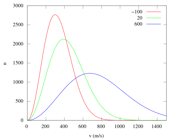
M-B distribution (from [Wikipedia](https://commons.wikimedia.org/wiki/File:Maxwell-Boltzmann_distribution.svg)).
With all these pieces of information, we can perform a simulation in a, so called, NVE ensemble 2, where the number of particles, the volume and the total energy of the system is conserved.
But usually, we want to compute quantities that are experimentally measured. And in experiments what is fixed is not the energy but the temperature, or not the volume but the pressure.
Therefore, we need to introduce two new ingredients that will be explained in the theoretical lessons: a thermostat and a barostat. These two pieces will help us in simulating our system in the correct ensemble, NVT and NpT.
An ingredient that is not evident from the above discussion is the necessity to reproduce experimental results.
The workflow of your simulation would look like this:
- build the setup:
- minimise the system;
- equilibrate the system in NVT;
- equilibrate the system in NpT;
- go back to NVT to reduced the perturbation introduced in your system.
Depending on the system, step 5 may not be performed.
BPTI
The bovine pancreatic trypsin inhibitor is a small protein extensively studied since the dawn of Molecular Dynamics. It inhibits the enzyme trypsin, responsible for the protein digestion.
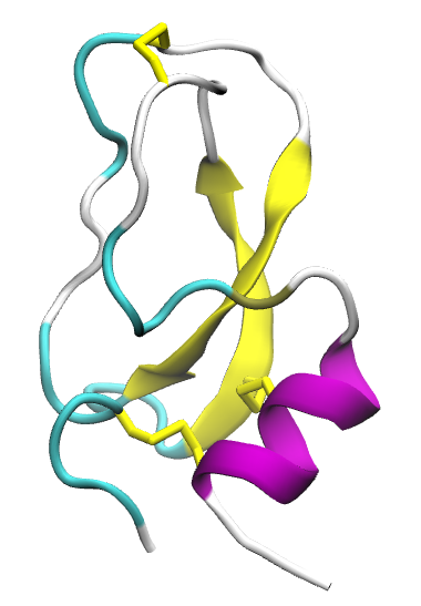
It was the first macromolecule of biological relevance simulated with MD with the seminal paper Dynamics of folded proteins by McCammon, Gelin and Karplus.
The BTPI binds the trypsin hindering the ability of cleaving other proteins. For more details, see the Notes.
Load the complex in the bpti_trypsin/ folder and check the LYS15 of the bpti.
PSF
Let’s start from the pdb of the protein alone from the previous tutorial.
We will build again the psf with the AutoPSF plugin.
Open VMD in your working folder tutorial3, and load your pdb file.
Now go to Extension -> Modeling
-> Automatic PSF Builder.
A new window pops up:
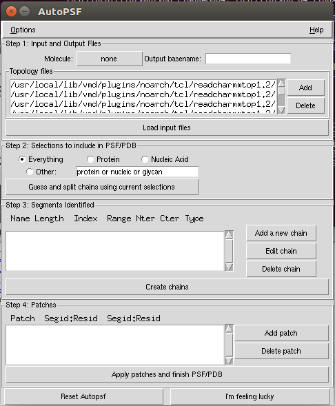
If you click on Options, you see some flags.
This leads us to a small correction to what was said last time.
When building the psf, the position of the angles and dihedrals are
recomputed according to the topology file. Therefore the minimisation has
less impact on matching the pdb coordinates with the ideal 3D arrangement.
Still do the minimisation for the steric clashes!
The steps we will perform is:
- Check if our molecule is properly loaded;
- Select the output name or use the default one;
- Delete the default
top*files and add our own; - Load the input files;
- Guess and create the chains;
- Check if our patches are automagically imported;
- Finish the psf.
Check the correctness of the patches!
It will create and load a new molecule, both psf and pdb.
Implicit solvent
Last time we performed few time steps of a simulation in vacuum. Of course, proteins do not live in the outer space in a galaxy far, far away… (unless we are studying Midi-chlorian, ça va sans dire).
Proteins live in an aqueous environment, with ions, all kinds of ligands and so on and so forth. We would like to mimic as good as possible the biological environment by adding explicitly water molecules. This will be done in few steps. But in this section we will use an implicit solvent model.
Implicit Solvent model is a computational technique that introduces many effects due to solvent-solute interactions, such as screening effects, without using the water atoms. Removing the water molecules accelerates the simulation both in the exploration of the solute conformations, and in the CPU time required to actually do the computation.
Implicit models are less accurate than the explicit counterpart!
In particular we will use the Generalised Born implicit solvent (GBIS) model. The details are left for the theoretical part of the course. The main idea is to screen more the atoms nearby the surface of the protein nearby the solvent (and give them a small effective radius) and the opposite for the buried atoms inside the protein.
The parameters that we have to set are:
gbis yes: we want to use the GBIS;cutoff 14: for the electrostatic interactions (in Angstrom);alphaCutoff 12: to determine the appropriate radius (in Angstrom);ionconcentration: the default value is0.2.
Let’s open the configuration file for this simulation and see what is inside.
The section we will not discuss are defined by
# <--!
...
# !-->
Fix the lines left blank in the configuration file, and then launch the simulation.
This time we will slightly modify the launching command:
$ namd2 +p2 conf.namd > bubu.log &
To check how much time the program needs, type in the shell:
$ grep "^TIMING" bubu.log
For 100k steps it will take 20 minutes.
Several files will be dumped from NAMD:
.logfile;.dcd: trajectory;.restart.*: to restart the simulation;.coor: binary for coordinates;.vel: binary for velocities;.xsc/.xst: for the simulation box;
Let’s start from the .log file.
Let’s open it with ViM. There is a lot of information written in it, such as
the initialisation of the system, checking the number of atoms, the existence of the
files, the correctness of the parameters file, the recap of the setup defined
in the configuration file.
Search the word Benchmark. The data you find here are useful to establish
the amount of resources (CPU/GPU) you should use.
Then we can check the thermodynamic quantities we asked to compute on the fly.
They will be written as row each defined timestep.
The keywords are ETITLE to have the headers of the columns, and ENERGY
for the actual values.
While the simulation is running, you can write a tcl script to compute the
Root mean square displacement of the protein. It is defined as, assuming
that all the atoms have the same mass:
Usually it is performed considering only the C\(\alpha\) and the following procedure is followed:
- Align the structure of each frame to the first frame structure, in order to remove the roto-translation of the system;
- Compute the RMSD.
This quantity gives a qualitative estimate of the convergence of the simulation. We can define two segments of the total simulated time:
- an equilibration phase that allows the system to reach the “"”equilibrium”””
- a production phase from which we will compute the data we want.
A criterion to check the equilibration of a system is to check for a plateau in the rmsd.
Write the rmsd.tcl script
Once the simulation is completed, let’s analyse the output in the .log file.
In VMD go in Extension -> Analysis -> NAMD Plot.
You should see this:
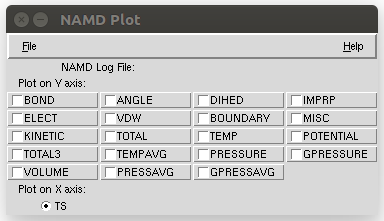
Load the .log file and analyse the TEMP.
Can you explain the behaviour of the temperature?
.
We can also save the extracted info, but it is too cumbersome (imho).
So let’s use the shell.
The idea is to extract from the log file some lines. We will use the following
commands:
$ grep "^ETITLE" bubu.log |
tail -n 1 > thermo.dat
$ grep "^ENERGY" bubu.log > > thermo.dat
See if the file is properly written. And now let’s plot something.
$ gnuplot
> set key autotitle columnheader
> p "thermo.dat" u 2:13 w l
Check the potential energy 14, the total energy 12.
Compare in the same plot the temperature 13 with the average temperature 16.
A longer trajectory (10 ns) in implicit solvent is available here.
Explicit Solvent
If we want to simulate a protein in a water box, we should build a water box («Elementary, my dear Watson!»).
The idea is to create a box
To do so, we can use the solvate package in VMD. In the Tk console:
% solvate
and let’s see the option we can use.
Solvate the system!
Rotate the system and add a padding of 9 Angstrom.
The water box will define also our simulation box, a cube. Since we will use the periodic boundary conditions, we do not want that the protein interacts with its own image, so we cannot choose a padding too small. The protein should be at least 14 A from its image.
This at least works only for this tutorial. For production runs, you should take into account the autocorrelation of the water molecules with themselves. Therefore, as a rule of thumb, you should use a padding of 18 A. Of course you can use a padding of 50 A, but it is a waste of resources.
To perform a visual check, be sure that your solvated molecule is loaded as top. Let’s first shift to the center of the box with the command:
% set all [atomselect top "all"]
% $all moveby [vecinvert [measure center $all]]
% $all writepdb solvated_centered.pdb
We wrote down the new coordinates because they will be useful in the following.
Now that the protein is centered in (0,0,0), let’s measure the extension of
box:
% measure minmax $all
This command gives us the x_min, y_min, z_min and x_max, y_max, z_max of
the box. Taking the difference along each axis, \(\Delta x\) etc,
gives use the three sizes of the box.
Let’s tell VMD what the unit cell looks like:
% molinfo top set a _..._
% molinfo top set b _..._
% molinfo top set c _..._
and visualise the images. Go to Graphics -> Representation -> Periodic and
put a tick in -X +X -Y +Y.
You can also measure the distance between atoms with the usual command 2.
Once the visual inspection is done, we would like to add ions, too. ““Why do we need ions?” I hear you ask…
There are two reasons for ions. The trivial one is because there are ions in solution in cells. The obscure, for now, reason is related to computation of the electrostatic interactions. But it will be clearer later in the course ;)
This time we will use the GUI to ionise the system.
First delete all the loaded molecules, and reload the psf and the new pdb.
Go to Extension -> Modeling -> Try-to-guess.
We will neutralise the charge in the system and add a 0.1 M ion concentration.
Why is our system charged in the first place?
Further Notes
- NAMD User guide
- Molecular Modeling of Proteins, edited by Andreas Kukol.
Notes
-
This tutorial is based on NAMD tutorial (Unix version, but there is also a Windows version) and BPTI case study. ↩
-
Please notice it is written with the e, ensemble. ↩