
In this session we will build the setup for an explicit solvent simulation, analyse the configuration file, launch it on a cluster, and perform a small analysis of a system.1
Question time, again
Let’s recap the so called MD machinery.
What files do we need?
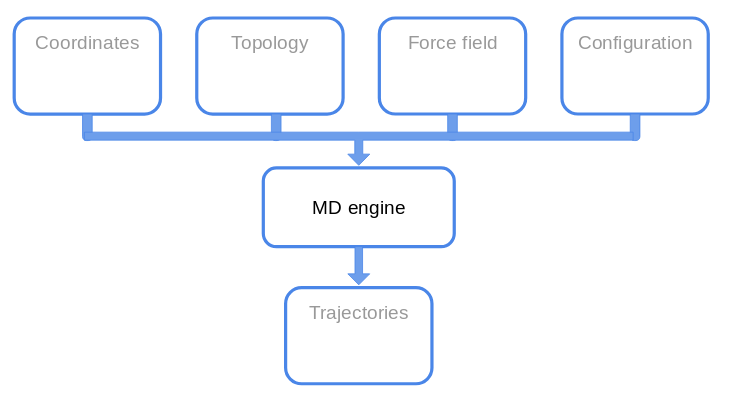
Recap of last tutorial
Last time we built the setup for an explicit solvent simulation.
What steps did we follow?
Explicit solvent (part 2)
Let’s run the simulation. As a guideline, let’s remind the procedure we should follow for a production simulation:
- minimisation;
- heavy atoms of the protein harmonically restrained to their starting positions while the solvent equilibrates around the protein;
- NVT simulation to go into the canonical ensemble;
- Add the pressure.
We will run an NpT simulation just to get accustomed to the new option. You already know what lines you should fill, but now we have two more things to add.
Use the centered box!!!
First, now our system has also water molecules, therefore we need a new parameter file. It’s in the VMD plugin folder.
Second, we have to set the center and the a b c of the box.
The center should be 0.0 0.0 0.0 because of one of the previous commands,
and the cellVectors are
cellBasisVector1 _Delta x_  0.0  0.0
cellBasisVector2   0.0   _Delta y_ 0.0
cellBasisVector3   0.0  0.0  _Delta z
Thermostat
To perform an NVT simulation, we need to use a thermostat. For NAMD, the algorithm we will employ is the Langevin thermostat:
\[m \frac{d^2 x}{dt^2} = -\nabla U(x) - \gamma \frac{dx}{dt} + \sigma \xi\]where \(\gamma\) is the damping coefficient, \(\xi\) is a random number with 0 mean and standard deviation 1. The parameter \(\sigma\) is related to the damping coefficient by the fluctuation-dissipation theorem:
\(\sigma^2 = 2 k_B T m \gamma\).
What we will set is the damping coefficient \(\gamma\) (1/ps). The higher the value of this coefficient, the smaller are the fluctuations of the temperature. But then the system is highly perturbed. As a rule of thumb, the value of \(\gamma\) should be set to the smallest In general, a value between 1 and 10 ps\(^{-1}\) should be fine. value that preserves the wanted temperature (on average).
We have also an option to couple the thermostat to the hydrogen atoms of the system. Since we constrain the same atoms, we will disable it.
Launching the simulation
First launch the simulation with 1 core:
$ namd2 conf.namd > lognameN.log &
Does it work?
$ What is the problem related to?
Now try to launch namd using more cores:
$ namd2 +pN conf.namd > lognameN.log &
where N is the number of cores available.
Launch the same simulation using 2,3,4 processes (change also the logfile name).
In general you should be able to run with 4 cores,
but remember that your computer needs some resources for the
opetating system. Therefore, you may not see an increase in the performances
for 3 processes to 4.
1) The output will be overwritten.
2) If you want to do a for-loop modify the command above (hint:`&`)
This time with 4 cores, the simulation takes ~50min for 100k steps. So, launch 1000 time steps of simulation to check if it works.
A longer trajectory (10 ns) in explicit solvent is available here.
AWK detour
AWK is a scripting language to manipulate text. It is particular useful for small tasks that do not rqeuire a lot of lines of code.
The basic syntax of an awk instruction is:
awk ' condition {some actions}' < input.file.
awk will loop over the lines of the file and perform the actions you wrote,
if condition is satisfied. No condition implies True.
The default variables you will need are:
NF: number of fields (i.e. columns separated as default by blank spaces);NR: number of rows (i.e. lines), the counter over which the default loop is performed;$0: a whole line;$i: the i-th field; Moreover you can do operations before (BEGIN) and after (END) the main loop.
First, create a file with 1 column filled with numbers from 1 to 100. Hint: use a bash for-loop.
Then, let’s compute the sum and the average.
awk 'BEGIN{sum=0} {sum += $1} END{print "sum:", sum, "\navg:", sum/NR}' < gauss_spicciame_casa.dat
See Notes for more information and fancy things2.
Now that we know a bit of awk, let’s use it for our purposes. First let’s see how different numbers of cores affect the computation.
$ grep "Benchmark" logname1.log | awk '{print $X, $Y, $Z}' > benchmark.dat
Of course we can do the same for all the 4 logfiles.
When do you have the ""best"" perfomances?
We saw the TIMING and Benchmark lines.
What is the difference according to you?
We can also use awk to get rid of the unwanted columns in the thermo.dat
we obtained before.
Make a file with timestep and temperature only,
using awk.
Try to compute the average of the same two quantities for the "equilibrated"
part with _awk_
Excursus
VadeVecum for HPC Unitn
ovvero
Read Me before using the cluster
This is a very small guide about launching jobs on HPC@Unitn. It is meant to be helpful for the master students who attended Computational Biophysics.
You are supposed to have a basic knowledge of bash scripting language (i.e.
cd, ls, mkdir and so on…) and a decent OS (i.e. not Windows).
For more info about the cluster, see HPC website. For more info about how to use the cluster and the batch scheduler, see section 2.
Important: the backslash \ at the end of a line in a code block means
that the line continues to the next line. Therefore, if you find
echo "Ciao, sono un \
pokemon"
you have to write in your file:
echo "Ciao, sono un pokemon"
1. How to connect
In order to connect to the HPC cluster, you have to be connected to the university network:
- you are connected to Unitn-x or similar (so you are in one of the university structures);
- if you log from home, you need to use the university VPN (install the Pulse secure and google how to connect to unitn).
Once one of the aforementioned criteria is fulfilled, then open a shell (Ctrl+Alt+t for Linux user) and type:
ssh <your-unitn-username>@hpc2.unitn.it
and then your password will be requested.
NOW you are connected to the login computers. DO NOT LAUNCH JOBS THERE: those computers are meant just for the job submission, since they are shared among all connected users and they have to be available. If you want to do something on the fly, using only few cores for few minutes, go interactively (see 2.1.3)
2. How to launch a job
The cluster has a batch scheduler, a software that organises the execution of the jobs coming from different users with different requested resources.
Basic dictionary (probably wrong):
- core: part of a computer that does things
- node: the whole computer (with multiple cores in it) connected with other computers with an ethernet cable;
- walltime: maximum time you will be granted; if your job is not ended yet, it will be killed. So, choose it carefully and use the
BenchmarkNAMD provides you for a good estimate.
On HPC@Unitn each node has a variable number of cores. We will use only the nodes with GPUs.
We remind you that you should request maximum 20 cores (Herr Professor Doktor said 16, but at most ask for 20 without telling him). As far as I know, you will not be able to run, statistically, those jobs that request more than 10 cores per nodes. Therefore, either you ask for 10 cores only on a single node (the following line will be clear in a while):
#PBS -l select=1:ncpus=10:mpiprocs=10:mem=40GB
or you ask for 10 cores on two nodes (using then 20 cores in total)
#PBS -l select=2:ncpus=10:mpiprocs=10:mem=40GB
IMPORTANT: before launching THE simulation, just run small simulations (1000 timesteps maximum) asking for different numbers of cores. For example: launch 3 simulations requesting 5, 10 e 20 cores (ça va sans dire, set the walltime at 10 mins). Depending on your system, you will have a small gain in performances using 20 cores with respect to 10 cores. If this is your case, use only 10 cores, since it will speed up your time in queue.
2.1 What to do in practice
In practice we will use the nodes with gpus to perform our computation.
We will monitor your usage of the cluster.
Any not appropriate usage will be reported to the Admins and to the professor.
2.1.0 Install NAMD
First we need to download NAMD in the CUDA version (multicore).
When the download is completed, you can upload your file to the home/ of your
account using:
$ scp file your_username@hpc.unitn.it:
As for your local version of NAMD, you have to install it (just extract it) and
create an alias in your (on the cluster) home.
scp works as cp: if you want to upload or download a folder you have to use
the option -r.
Please note the : at the end of the command: the colon represents your home.
If you want to save a file in another directory you should use
$ scp file your_username@hpc.unitn.it:path/to/a/folder
With a slight modified version of the command above you can upload all the files you need to perform the simulation.
What files do you need?
2.1.1 Create batch file
Go to your working folder, where you have the configuration file of namd,
the .psf .pdb files and so on, and create a submit_me.pbs file as
described below (the extension pbs is purely formal).
#!/bin/bash
#PBS -l select=1:ncpus=10:mpiprocs=10:mem=10GB
#PBS -l walltime=00:10:00
#PBS -q short_gpuQ
#PBS -N USE_AN_APPROPRIATE_NAME
#PBS -o appropriate_name_out
#PBS -e appropriate_name_err

# This is a comment.
# From the /home in the compute node we move to the
# directory from which we launched the job
# (and where you, hopefully, have your files)

cd $PBS_O_WORKDIR

namd2 +p10 +setcpuaffinity +devices 0 conf.namd > log.log
After the file is ready, you submit the job with:
qsub submit_me.pbs
Now you can wait, have a cup of coffee and pray.
2.1.2 What to modify
All the lines starting with #PBS are NOT comments but instructions for
the batch scheduler.
#PBS -l select=<numberOfNodes>:ncpus=<numberOfCoresPerNode>\
:mpiprocs=<sameNumberOfNcpus>:mem=<GBofRAMnecessary>

#PBS -l walltime=hours:minutes:seconds

#PBS -q <queue to be used>

#PBS -N <name to be visualised using qstat>

#PBS -o/e <file to redirect stdout and stderr>
2.1.3 Interactive job
On the login shell type:
qsub -I -q <queue> -l select=1:ncpus=2:mpiprocs=2:mem=10GB,walltime=00:30:00
and then you can use the same commands you use in the submit_me.pbs file.
2.1.4 Check your job
To check the status of your submitted jobs, type in the shell:
qstat -u $USER
2.2 Further info
For more commands and the use of the batch scheduler:
- go to HPC@Unitn guide;
- type
man qsubin your login shell, aka RTFM.
Questions
For any technical questions, first check online (Google and StackOverflow are your best friends).
If in doubt, feel free (but not so free) to send me an e-mail:
gianfranco.abrusci@unitn.it
Trivial questions, already discussed during the tutorial lessons, will be answered in a formally non-polite way.
Go HAM on the cluster
Now you should have all the tools to perform a benchmark of your system. Use 2/5/10 cores to simulate 1000 steps of your system.
Is there any difference?
Compare the benchmark for the 2 cores with and without gpus.
Explicit vs Implicit
Let’s compute the RMSD for the simulation with explicit solvent. Perform the average of the temperature for the two kinds of simulations.
Compute the radius of gyration of the protein in implicit and explicit solvent.
Notes
-
See tutorial 3 for the references. ↩
-
Rtfm on
man awk, or use Google/StackOverflow. ↩