
All-atom simulations
Up to now, we saw a fair range of all-atoms simulations. Each atom is treated like a point-like particle; if constraints are used, we can set a 2 fs timestep.
With the help of a nice cluster, we can simulate a biological system for a reasonable amount of time (hopefully up to microseconds).
Let’s remind us the time-scale we are dealing with:
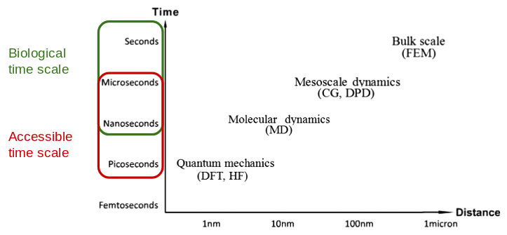
It would be nice to explore larger time scales and bigger systems. One way to do it is to coarse grain our system.
Coarse graining
A coarse-grained model is tool to simplify a system and study it at a lower level of details. Some degrees of freedom are integrated out and a group of atoms are represented by interaction sites:
\[\textbf{R}_I = \textbf{M}_I(\textbf{r}) = \sum_i c_{Ii}\textbf{r}_i\]where \(\textbf{R}\) is the CG site, and \(\textbf{M}\) is the mapping function.
The mapping can use a bottom-up or a top-down approach, can be modelled on a particular system or can be transferable to others. The definition of the interactions among sites is non trivial as well.
The aim of this page is not to treat the CG from a theoretical point of view. Several papers and books can be found on this topic1.
Shaken, not stirred
Let’s use one of the resources to perform a coarse-grained simulation: MARTINI.

I know you all like alcohol, but the name is related to a tower in Groningen, the Martini tower indeed, as an homage to the city in which this forcefield has been developed.
Martini uses a top-down approach to model the sites (now referred as beads) and their interactions. It is developed to reproduce structural or thermodynamical properties, still preserving a chemical specificity that allow the reproduction of experimental measurable quantities.
Initially, it was intended for lipids, then it was expanded to proteins. The current version is 2.2, and a version 3.x is currently in open beta.
‘Philosophy’ behind
The Martini ff in based on a 4 to 1 correspondence of atoms to beads.
Here, you can find a schematic representation of how the change in
resolution is performed:
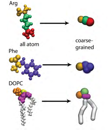
Also water is coarse-grained: four water molecules are set to one water bead.
Since the idea behind Martini is to be system independent, the mapping is done on a residue base, so that it is transferable.
Each amino acid is represented by one bead for the backbone and one or more for the sidechains.
Are all the CG residues defined in this way?
Depending on the sidechains, the beads are divided into four classes:
- charged: Q;
- polar: P;
- non polar: N;
- apolar: C.
These main classes have also subclasses to further differentiate the residues.
Each bead has 72 or 45 atomic mass units, regardless of the actual mass of the atoms they represent.
Force field
In Martini we have bonded interactions:
$$ \begin{align*} V_b & = \frac{1}{2} K_b (d_{ij}-d_b)^2\\ V_a & = \frac{1}{2} K_a \big[\cos(\phi_{ijk})-\cos(\phi_a)\big]^2\\ V_d & = K_d \big[1+\cos(\theta_{ijkl}-\theta_d)\big]\\ V_{id} & = K_{id} (\theta_{ijkl} - \theta_{id})\\ \end{align*} $$
Does it have the CHARMm functional form?
For the non-bonded interaction, the Lennard-Jones 12-6 potential is implemented and the electrostatic interaction with a dielectric constant of \(\epsilon_{diel} = 15\).
With the decrease in the number of particles to be simulated it comes the increase in the timestep that can be used.
As a rule of thumb, the timestep allowed by Martini is between 20 to 40 fs. The conservation of the total energy should be checked for the different time steps (keep in mind that the energy conservation depends also on other parameters).
Application and limitations
The advantage of a CG represention, specifically for Martini, can be employed to study several problems. A review of such topics can be found in the ‘Further notes’ section.
The speed-up in computation and the broader range of systems you could study are interesting features, but we need to remind ourselves that
From great power it comes greater responsabilities
or, like Ohm’s oncle said:
Therefore, limitations are to be taken into account. We already saw that the backbone of each residue is represented by a bead.
How would you represent alpha helices in this way?
You need to enforce the secondary structure.
A more subtle problem is the freezing of water at \(290\pm5 K\) due to the LJ 12-6 potential. So we need to add antifreezing water molecules. Due to this behaviour, systems that present water/air interfaces cannot be studied.
Tutorial
Let’s get started with the tutorial.
Go to the TCBG tutorial page and download the Residue-based Coarse-graining.
Once you are ready, put the green sticker on your laptop. DEMACIAAAAAAAA
Further readings
Papers on Martini: