Most of the scripts are taken from the MDAnaysis github repository. ASAP I will put the link, but a search will show you all the sources.
Introduction
After the simulation is completed, we need to analyse the trajectory.
There is plenty of tools you can use to perform the analysis.
Of course, VMD and Tcl scripting with the built-in functions of VMD, almost independent of the file format. Another option is to use Gromacs’ analysis tools, which require a specific format of the trajectory.
Today we will use Python as programming language, and the libraries MDAnalysis and prody. As usual, there are several options in the same Python environment
- MDtraj
- PyEmma
- others…
You can also use R and the package Bio3D.
Today’s tutorial is a mash-up of different tutorial available online.
CAVEAT: the terminology will likely be inexact. Let me know if you find any bugs and/or wrong information.
import numpy as np
import matplotlib.pyplot as plt
%matplotlib inline
MDAnalysis
If you are interest in the project, I link here the link to its website. The package is in development, with stable releases, and you can also contribute via Github with issues or pull request.
First of all we need to import the package:
import MDAnalysis as mda
mda.__version__
'0.19.2'
In order to deal with the trajectory, or with a single pdb file, we need to create a Universe.
As for VMD, this Universe requires a topology and a coordinate file.
Let’s first define the two files and then let’s create the Universe.
%ls
PSF = 'adk_equilibrium/adk4AKE.psf'
eqDCD = 'adk_equilibrium/1ake_007-nowater-core-dt240ps.dcd'

u = mda.Universe(PSF, eqDCD)
What is u?
u
<Universe with 3341 atoms>
u.trajectory.n_frames
4187
u.atoms
<AtomGroup with 3341 atoms>
u.atoms.dimensions
array([85.53471, 85.53471, 85.53471, 90.     , 90.     , 90.     ],
      dtype=float32)
Selecting atoms
It is possible to select only a subset of atoms.
alanines = u.select_atoms('resname ALA')
alanines
<AtomGroup with 190 atoms>
alanines.resids
array([  8,   8,   8,   8,   8,   8,   8,   8,   8,   8,  11,  11,  11,
        11,  11,  11,  11,  11,  11,  11,  17,  17,  17,  17,  17,  17,
        17,  17,  17,  17,  37,  37,  37,  37,  37,  37,  37,  37,  37,
        37,  38,  38,  38,  38,  38,  38,  38,  38,  38,  38,  49,  49,
        49,  49,  49,  49,  49,  49,  49,  49,  55,  55,  55,  55,  55,
        55,  55,  55,  55,  55,  66,  66,  66,  66,  66,  66,  66,  66,
        66,  66,  73,  73,  73,  73,  73,  73,  73,  73,  73,  73,  93,
        93,  93,  93,  93,  93,  93,  93,  93,  93,  95,  95,  95,  95,
        95,  95,  95,  95,  95,  95,  99,  99,  99,  99,  99,  99,  99,
        99,  99,  99, 127, 127, 127, 127, 127, 127, 127, 127, 127, 127,
       176, 176, 176, 176, 176, 176, 176, 176, 176, 176, 186, 186, 186,
       186, 186, 186, 186, 186, 186, 186, 188, 188, 188, 188, 188, 188,
       188, 188, 188, 188, 194, 194, 194, 194, 194, 194, 194, 194, 194,
       194, 203, 203, 203, 203, 203, 203, 203, 203, 203, 203, 207, 207,
       207, 207, 207, 207, 207, 207, 207, 207])
The information stored in the universe are numpy array. So you can apply all the modules in numpyu
np.unique(alanines.resids)
array([  8,  11,  17,  37,  38,  49,  55,  66,  73,  93,  95,  99, 127,
       176, 186, 188, 194, 203, 207])
You can also use wildcards in the select_atoms string, or use the slicing.
carbons = u.select_atoms('name C*')
carbons.names
array(['CA', 'CB', 'CG', ..., 'C', 'C', 'CA'], dtype=object)
carbons[:10].names
array(['CA', 'CB', 'CG', 'CE', 'C', 'CA', 'CB', 'CG', 'CD', 'CZ'],
      dtype=object)
carbons and carbons[:10] are Atomgroup.
carbons
<AtomGroup with 1040 atoms>
RMSD
In order to establish equilibration, the first thing to check is equilibration.
I remind you that the RMSD is defined as \(RMSD(t) = \sqrt{\frac{\sum_i m_i(\vec{r}_i(t) - \vec{r}_i(t_0))^2}{\sum_i m_i}}\)
u.trajectory.frame
0
The hard way
We want to compute RMSD. There is a built-in function in MDAnalysis, called rmsd.
from MDAnalysis.analysis.rms import rmsd
PBD_closed = 'adk_equilibrium/adk_closed.pdb'
ref = mda.Universe(PSF, PDB_closed)
ref
<Universe with 3341 atoms>
mobile = mda.Universe(PSF, eqDCD)     # we use the first frame
mobile.trajectory.frame
0
Let’s compute the rmsd.
rmsd(mobile.select_atoms('name CA').positions, ref.select_atoms('name CA').positions)
29.017277853848036
Let’s visualise the two structures in VMD. They do not look so different. Moreover they have the same conformation (closed).
Probably we should investigate better how rmsd works.
help(rmsd)
Help on function rmsd in module MDAnalysis.analysis.rms:

rmsd(a, b, weights=None, center=False, superposition=False)
    Returns RMSD between two coordinate sets `a` and `b`.

    `a` and `b` are arrays of the coordinates of N atoms of shape
    :math:`N times 3` as generated by, e.g.,
    :meth:`MDAnalysis.core.groups.AtomGroup.positions`.

    Note
    ----
    If you use trajectory data from simulations performed under **periodic
    boundary conditions** then you *must make your molecules whole* before
    performing RMSD calculations so that the centers of mass of the mobile and
    reference structure are properly superimposed.


    Parameters
    ----------
    a : array_like
        coordinates to align to `b`
    b : array_like
        coordinates to align to (same shape as `a`)
    weights : array_like (optional)
        1D array with weights, use to compute weighted average
    center : bool (optional)
        subtract center of geometry before calculation. With weights given
        compute weighted average as center.
    superposition : bool (optional)
        perform a rotational and translational superposition with the fast QCP
        algorithm [Theobald2005]_ before calculating the RMSD; implies
        ``center=True``.

    Returns
    -------
    rmsd : float
        RMSD between `a` and `b`

    Notes
    -----
    The RMSD :math:`\rho(t)` as a function of time is calculated as

    .. math::

       \rho(t) = \sqrt{\frac{1}{N} \sum_{i=1}^N w_i \left(\mathbf{x}_i(t)
                                - \mathbf{x}_i^{\text{ref}}\right)^2}

    It is the Euclidean distance in configuration space of the current
    configuration (possibly after optimal translation and rotation) from a
    reference configuration divided by :math:`1/\sqrt{N}` where :math:`N` is
    the number of coordinates.

    The weights :math:`w_i` are calculated from the input weights
    `weights` :math:`w'_i` as relative to the mean:

    .. math::

       w_i = \frac{w'_i}{\langle w' \rangle}


    Example
    -------
    >>> u = Universe(PSF,DCD)
    >>> bb = u.select_atoms('backbone')
    >>> A = bb.positions.copy()  # coordinates of first frame
    >>> u.trajectory[-1]         # forward to last frame
    >>> B = bb.positions.copy()  # coordinates of last frame
    >>> rmsd(A, B, center=True)
    3.9482355416565049

    .. versionchanged: 0.8.1
       *center* keyword added
    .. versionchanged: 0.14.0
       *superposition* keyword added
# Removing translations
rmsd(mobile.select_atoms('name CA').positions, ref.select_atoms('name CA').positions, center=True)
22.39150433851966
# Removing the rotation
rmsd(mobile.select_atoms('name CA').positions, ref.select_atoms('name CA').positions,
     center=True, superposition=True)
1.8181973717315183
We are usually interested in the RMSD during all the trajectory.
Let’s do that!
The idea is to loop over the trajectory. The positions of our selection are updated as me move along the trajectory.
mobile_selection = mobile.select_atoms('protein and name CA')
ref_selection = ref.select_atoms('protein and name CA')

for ts in mobile.trajectory[:10]:
    print(ts)
< Timestep 0 with unit cell dimensions [85.53471 85.53471 85.53471 90.      90.      90.     ] >
< Timestep 1 with unit cell dimensions [85.69929 85.69929 85.69929 90.      90.      90.     ] >
< Timestep 2 with unit cell dimensions [85.61096 85.61096 85.61096 90.      90.      90.     ] >
< Timestep 3 with unit cell dimensions [85.58586 85.58586 85.58586 90.      90.      90.     ] >
< Timestep 4 with unit cell dimensions [85.6257 85.6257 85.6257 90.     90.     90.    ] >
< Timestep 5 with unit cell dimensions [85.66024 85.66024 85.66024 90.      90.      90.     ] >
< Timestep 6 with unit cell dimensions [85.61478 85.61478 85.61478 90.      90.      90.     ] >
< Timestep 7 with unit cell dimensions [85.636696 85.636696 85.636696 90.       90.       90.      ] >
< Timestep 8 with unit cell dimensions [85.63573 85.63573 85.63573 90.      90.      90.     ] >
< Timestep 9 with unit cell dimensions [85.621025 85.621025 85.621025 90.       90.       90.      ] >
computedRMSD = []
for ts in mobile.trajectory[:]:
    computedRMSD.append(rmsd(mobile_selection.positions, ref_selection.positions,
                             center=True, superposition=True))
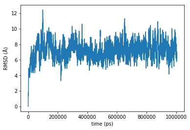
plt.plot(computedRMSD);
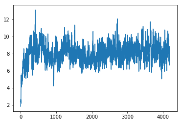
On the x-axis we have the indices of the list. Of course we can easily modify the label if we know what is the timestep of the simulation.
mobile.trajectory.dt
240.00000489999024
The easy way
We can take advantage of more built-in functions in MDAnalysis.
from MDAnalysis.analysis.base import analysis_class

help(analysis_class)
Help on function analysis_class in module MDAnalysis.analysis.base:

analysis_class(function)
    Transform a function operating on a single frame to an analysis class

    For an usage in a library we recommend the following style:

    >>> def rotation_matrix(mobile, ref):
    >>>     return mda.analysis.align.rotation_matrix(mobile, ref)[0]
    >>> RotationMatrix = analysis_class(rotation_matrix)

    It can also be used as a decorator:

    >>> @analysis_class
    >>> def RotationMatrix(mobile, ref):
    >>>     return mda.analysis.align.rotation_matrix(mobile, ref)[0]

    >>> rot = RotationMatrix(u.trajectory, mobile, ref).run(step=2)
    >>> print(rot.results)
Let’s assume we have a function that works only on one frame.
def my_rmsd(mobile_ag, ref_ag):
    '''We always want to align the trajectory to the reference frame. So we set
        center = True
        superposition = True
    '''
    return rmsd(mobile_ag.positions, ref_ag.positions, center=True, superposition=True)
my_rmsd
<function __main__.my_rmsd(mobile_ag, ref_ag)>
my_rmsd(mobile_ag=mobile.select_atoms('name CA'), ref_ag=ref.select_atoms('name CA'))
1.8181973717315183
@analysis_class
def my_rmsd(mobile_ag, ref_ag):
    '''We always want to align the trajectory to the reference frame. So we set
        center = True
        superposition = True
    '''
    mobile_pos = mobile_ag.positions
    return rmsd(mobile_pos, ref_ag.positions, center=True, superposition=True)
my_rmsd
MDAnalysis.analysis.base.analysis_class.<locals>.WrapperClass
a = my_rmsd(mobile.trajectory, mobile_ag=mobile.select_atoms('name CA'), ref_ag=ref.select_atoms('name CA')).run()
plt.plot(a.results)
[<matplotlib.lines.Line2D at 0x7f01b9da0c18>]
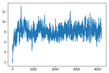
This is a nice way to extend a function that works on a frame to the whole trajectory. Of course we can do better, if there is already something that does that for us ;)
The lazy way
from MDAnalysis.analysis.rms import RMSD
help(RMSD)
Help on class RMSD in module MDAnalysis.analysis.rms:

class RMSD(MDAnalysis.analysis.base.AnalysisBase)
 |  Class to perform RMSD analysis on a trajectory.
 |
 |  The RMSD will be computed for two groups of atoms and all frames in the
 |  trajectory belonging to `atomgroup`. The groups of atoms are obtained by
 |  applying the selection selection `select` to the changing `atomgroup` and
 |  the fixed `reference`.
 |
 |  Note
 |  ----
 |  If you use trajectory data from simulations performed under **periodic
 |  boundary conditions** then you *must make your molecules whole* before
 |  performing RMSD calculations so that the centers of mass of the selected
 |  and reference structure are properly superimposed.
 |
 |
 |  Run the analysis with :meth:`RMSD.run`, which stores the results
 |  in the array :attr:`RMSD.rmsd`.
 |
 |  Method resolution order:
 |      RMSD
 |      MDAnalysis.analysis.base.AnalysisBase
 |      builtins.object
 |
 |  Methods defined here:
 |
 |  __init__(self, atomgroup, reference=None, select='all', groupselections=None, filename='rmsd.dat', weights=None, tol_mass=0.1, ref_frame=0, **kwargs)
 |      Parameters
 |      ----------
 |      atomgroup : AtomGroup or Universe
 |          Group of atoms for which the RMSD is calculated. If a trajectory is
 |          associated with the atoms then the computation iterates over the
 |          trajectory.
 |      reference : AtomGroup or Universe (optional)
 |          Group of reference atoms; if ``None`` then the current frame of
 |          `atomgroup` is used.
 |      select : str or dict or tuple (optional)
 |          The selection to operate on; can be one of:
 |
 |          1. any valid selection string for
 |             :meth:`~MDAnalysis.core.groups.AtomGroup.select_atoms` that
 |             produces identical selections in `atomgroup` and `reference`; or
 |
 |          2. a dictionary ``{'mobile': sel1, 'reference': sel2}`` where *sel1*
 |             and *sel2* are valid selection strings that are applied to
 |             `atomgroup` and `reference` respectively (the
 |             :func:`MDAnalysis.analysis.align.fasta2select` function returns such
 |             a dictionary based on a ClustalW_ or STAMP_ sequence alignment); or
 |
 |          3. a tuple ``(sel1, sel2)``
 |
 |          When using 2. or 3. with *sel1* and *sel2* then these selection strings
 |          are applied to `atomgroup` and `reference` respectively and should
 |          generate *groups of equivalent atoms*.  *sel1* and *sel2* can each also
 |          be a *list of selection strings* to generate a
 |          :class:`~MDAnalysis.core.groups.AtomGroup` with defined atom order as
 |          described under :ref:`ordered-selections-label`).
 |
 |      groupselections : list (optional)
 |          A list of selections as described for `select`, with the difference
 |          that these selections are *always applied to the full universes*,
 |          i.e., ``atomgroup.universe.select_atoms(sel1)`` and
 |          ``reference.universe.select_atoms(sel2)``. Each selection describes
 |          additional RMSDs to be computed *after the structures have been
 |          superimposed* according to `select`. No additional fitting is
 |          performed.The output contains one additional column for each
 |          selection.
 |
 |          .. Note:: Experimental feature. Only limited error checking
 |                    implemented.
 |      filename : str (optional)
 |          write RMSD into file with :meth:`RMSD.save`
 |
 |          .. deprecated:; 0.19.0
 |             `filename` will be removed together with :meth:`save` in 1.0.
 |
 |      weights : {"mass", ``None``} or array_like (optional)
 |           choose weights. With ``"mass"`` uses masses as weights; with ``None``
 |           weigh each atom equally. If a float array of the same length as
 |           `atomgroup` is provided, use each element of the `array_like` as a
 |           weight for the corresponding atom in `atomgroup`.
 |      tol_mass : float (optional)
 |           Reject match if the atomic masses for matched atoms differ by more
 |           than `tol_mass`.
 |      ref_frame : int (optional)
 |           frame index to select frame from `reference`
 |      verbose : bool (optional)
 |           Show detailed progress of the calculation if set to ``True``; the
 |           default is ``False``.
 |
 |      Raises
 |      ------
 |      SelectionError
 |           If the selections from `atomgroup` and `reference` do not match.
 |      TypeError
 |           If `weights` is not of the appropriate type; see also
 |           :func:`MDAnalysis.lib.util.get_weights`
 |      ValueError
 |           If `weights` are not compatible with `atomgroup` (not the same
 |           length) or if it is not a 1D array (see
 |           :func:`MDAnalysis.lib.util.get_weights`).
 |
 |           A :exc:`ValueError` is also raised if `weights` are not compatible
 |           with `groupselections`: only equal weights (``weights=None``) or
 |           mass-weighted (``weights="mass"``) are supported for additional
 |           `groupselections`.
 |
 |      Notes
 |      -----
 |      The root mean square deviation :math:`\rho(t)` of a group of :math:`N`
 |      atoms relative to a reference structure as a function of time is
 |      calculated as
 |
 |      .. math::
 |
 |         \rho(t) = \sqrt{\frac{1}{N} \sum_{i=1}^N w_i \left(\mathbf{x}_i(t)
 |                                  - \mathbf{x}_i^{\text{ref}}\right)^2}
 |
 |      The weights :math:`w_i` are calculated from the input weights `weights`
 |      :math:`w'_i` as relative to the mean of the input weights:
 |
 |      .. math::
 |
 |         w_i = \frac{w'_i}{\langle w' \rangle}
 |
 |      The selected coordinates from `atomgroup` are optimally superimposed
 |      (translation and rotation) on the `reference` coordinates at each time step
 |      as to minimize the RMSD. Douglas Theobald's fast QCP algorithm
 |      [Theobald2005]_ is used for the rotational superposition and to calculate
 |      the RMSD (see :mod:`MDAnalysis.lib.qcprot` for implementation details).
 |
 |      The class runs various checks on the input to ensure that the two atom
 |      groups can be compared. This includes a comparison of atom masses (i.e.,
 |      only the positions of atoms of the same mass will be considered to be
 |      correct for comparison). If masses should not be checked, just set
 |      `tol_mass` to a large value such as 1000.
 |
 |      .. _ClustalW: http://www.clustal.org/
 |      .. _STAMP: http://www.compbio.dundee.ac.uk/manuals/stamp.4.2/
 |
 |
 |      See Also
 |      --------
 |      rmsd
 |
 |
 |      .. versionadded:: 0.7.7
 |      .. versionchanged:: 0.8
 |         `groupselections` added
 |      .. versionchanged:: 0.16.0
 |         Flexible weighting scheme with new `weights` keyword.
 |      .. deprecated:: 0.16.0
 |         Instead of ``mass_weighted=True`` (removal in 0.17.0) use new
 |         ``weights='mass'``; refactored to fit with AnalysisBase API
 |      .. versionchanged:: 0.17.0
 |         removed deprecated `mass_weighted` keyword; `groupselections`
 |         are *not* rotationally superimposed any more.
 |      .. deprecated:: 0.19.0
 |         `filename` will be removed in 1.0
 |
 |  save(*args, **kwds)
 |      `save` is deprecated!
 |
 |      Save RMSD from :attr:`RMSD.rmsd` to text file *filename*.
 |
 |      Parameters
 |      ----------
 |      filename : str (optional)
 |          if no filename is given the default provided to the constructor is
 |          used.
 |
 |
 |
 |
 |
 |      .. deprecated:: 0.19.0
 |         You can instead use ``np.savetxt(filename, RMSD.rmsd)``.
 |         `save` will be removed in release 1.0.0.
 |
 |  ----------------------------------------------------------------------
 |  Methods inherited from MDAnalysis.analysis.base.AnalysisBase:
 |
 |  run(self, start=None, stop=None, step=None, verbose=None)
 |      Perform the calculation
 |
 |      Parameters
 |      ----------
 |      start : int, optional
 |          start frame of analysis
 |      stop : int, optional
 |          stop frame of analysis
 |      step : int, optional
 |          number of frames to skip between each analysed frame
 |      verbose : bool, optional
 |          Turn on verbosity
 |
 |  ----------------------------------------------------------------------
 |  Data descriptors inherited from MDAnalysis.analysis.base.AnalysisBase:
 |
 |  __dict__
 |      dictionary for instance variables (if defined)
 |
 |  __weakref__
 |      list of weak references to the object (if defined)
ca = mobile.select_atoms('protein and name CA')

R = RMSD(ca)
R.run()
<MDAnalysis.analysis.rms.RMSD at 0x7f01b9d9d668>
_, time, ca_rmsd = R.rmsd.T
plt.plot(time, ca_rmsd)
plt.xlabel('time (ps)');
plt.ylabel('RMSD (Å)');
ca_rmsd[0]
2.6076733666407134e-07
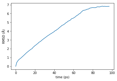
Compute the RMSD for the following trajectory neDCD = 'adk_equilibrium/adk_dims.dcd'
neDCD = 'adk_equilibrium/adk_dims.dcd'
u_ne = mda.Universe(PSF, neDCD, in_memory=True)
ca2 = u_ne.select_atoms('protein and name CA')

R2 = RMSD(ca2)
R2.run()
<MDAnalysis.analysis.rms.RMSD at 0x7f01b9d3e780>
_, time, ca_rmsd = R2.rmsd.T
plt.plot(time, ca_rmsd)
plt.xlabel('time (ps)');
plt.ylabel('RMSD (Å)');
RMSF
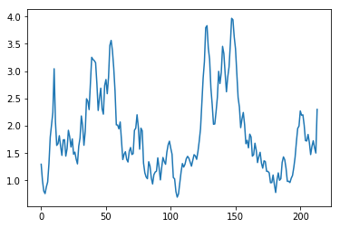
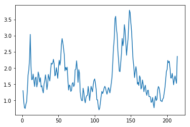
The RMSF is an equilibrium quantity that tells us how a certain atom fluctuates around its average position.
\[RMSF_i = \sqrt{ \langle (r_i - \langle r_i \rangle)^2 \rangle}\]Of course we have a built-in class.
from MDAnalysis.analysis.rms import RMSF
protein_heavy = mobile.select_atoms("protein and name CA")
myRMSF = RMSF(protein_heavy).run()
plt.plot(myRMSF.rmsf)
[<matplotlib.lines.Line2D at 0x7f01b30d7198>]
#help(RMSF)
We need to align the trajectory to a reference frame. We will use the open conformation.
from MDAnalysis.analysis import align

# Loading the structure
PDB_open = 'adk_equilibrium/adk_open.pdb'
open_uni = mda.Universe(PSF, PDB_open)
# Let's define a selection for the equilibrium universe
protein = mobile.select_atoms('protein')

# we PRE-align the structure
prealigner = align.AlignTraj(mobile=mobile, reference=open_uni,
                             select="protein and name CA", in_memory=True).run()

# Creating the reference (average) structure
reference_coordinates = mobile.trajectory.timeseries(asel=protein, start=1000).mean(axis=1)
# make a reference structure (need to reshape into a 1-frame "trajectory")
reference = mda.Merge(protein).load_new(
            reference_coordinates[:, None, :], order="afc")

#order afc is the way it returns the data array: a-tom, f-rame, c-oordinates
aligner = align.AlignTraj(u, reference, select="protein and name CA", in_memory=True).run(start=1000)
calphas = protein.select_atoms("name CA")
rmsfer = RMSF(calphas, verbose=True).run(start=1000)
Step 3187/3187 [100.0%]
plt.plot(calphas.resids, rmsfer.rmsf)
[<matplotlib.lines.Line2D at 0x7f01ba0dd978>]
Now we want to store the RMSF value in the beta field of a pdb. We can write the
open_uni.add_TopologyAttr(mda.core.topologyattrs.Tempfactors(np.zeros(len(u.atoms))))
protein = open_uni.select_atoms("protein")
len(protein.residues)
len(rmsfer.rmsf)
214
for residue, beta in zip(protein.residues, rmsfer.rmsf):
    residue.atoms.tempfactors = beta
protein.write("protein_with_bfactors.pdb")
/home/jarvis/anaconda2/envs/py3/lib/python3.6/site-packages/MDAnalysis/coordinates/PDB.py:902: UserWarning: Found no information for attr: 'altLocs' Using default value of ' '
  "".format(attrname, default))
/home/jarvis/anaconda2/envs/py3/lib/python3.6/site-packages/MDAnalysis/coordinates/PDB.py:902: UserWarning: Found no information for attr: 'icodes' Using default value of ' '
  "".format(attrname, default))
/home/jarvis/anaconda2/envs/py3/lib/python3.6/site-packages/MDAnalysis/coordinates/PDB.py:902: UserWarning: Found no information for attr: 'occupancies' Using default value of '1.0'
  "".format(attrname, default))
Radius of gyration
We already saw the radius of gyration:
\[R_\mathrm{gyr} = \sqrt{\frac{1}{M}\sum_{i=1}^{N} m_i(\mathbf{r}_i - \mathbf{R})^2}\]where $\mathbf{R}$ is the center of mass.
protein = mobile.select_atoms("protein")
Let’s investigate the methods for the AtomGroup protein.
rg = []
times = []
for ts in mobile.trajectory:
    rg.append(protein.radius_of_gyration())
    times.append(ts.time)
rg = np.array(rg)
times = np.array(times)
plt.plot(times, rg)
plt.title('Radius of gyration')
plt.xlabel("time (ps)")
plt.ylabel(r"$R_G$ (Å)");
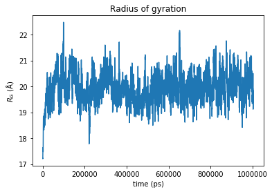
The radius of gyration behaves like the RMSD, and this is also an hint of how the equilibration can be considered reached.
Do the same for the ne_universe.
protein = u_ne.select_atoms("protein")
Let’s investigate the methods for the AtomGroup protein.
rg = []
times = []
for ts in u_ne.trajectory:
    rg.append(protein.radius_of_gyration())
    times.append(ts.time)
rg = np.array(rg)
times = np.array(times)
plt.plot(times, rg)
plt.title('Radius of gyration')
plt.xlabel("time (ps)")
plt.ylabel(r"$R_G$ (Å)");
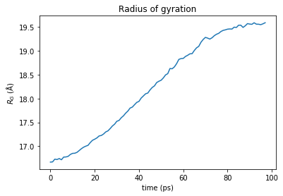
Contact map
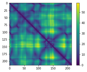
from MDAnalysis.lib import distances
Cα = open_uni.select_atoms('name CA')
d_CaCa = distances.distance_array(Cα.positions, Cα.positions)
fig, ax = plt.subplots()
img = plt.imshow(d_CaCa)
plt.colorbar(img);
Distances
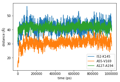
Experimental FRET labels: distances

- I52 - K145
- A55 - V169
- A127 - A194
Calculate the C$_\beta$ distances as proxies for the spin-label distances.
donors = mobile.select_atoms("name CB").select_atoms("resname ILE and resid 52",
                                           "resname ALA and resid 55",
                                           "resname ALA and resid 127")
acceptors = mobile.select_atoms("name CB").select_atoms("resname LYS and resid 145",
                                       "resname VAL and resid 169",
                                       "resname ALA and resid 194")
r = donors.positions - acceptors.positions
r
array([[ 20.777103,   7.352953, -23.57818 ],
       [ -8.003485,  -8.776337,  -8.839368],
       [ -9.672781, -28.934841,  -9.881233]], dtype=float32)
d = np.linalg.norm(r, axis=1)
d
array([32.27514 , 14.805887, 32.069088], dtype=float32)
def FRETdist(donors, acceptors):
    return np.linalg.norm(donors.positions - acceptors.positions, axis=1)
FRETdist(donors, acceptors)
array([32.27514 , 14.805887, 32.069088], dtype=float32)
distances = []
times = []
for ts in mobile.trajectory:
    d = FRETdist(donors, acceptors)
    distances.append(d)
    times.append(ts.time)
distances = np.array(distances)
times = np.array(times)
plt.plot(times, distances)
plt.legend(("I52-K145", "A55-V169", "A127-A194"))
plt.xlabel("time (ps)")
plt.ylabel(r"distance (Å)");
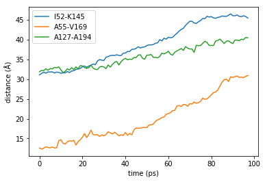
For the non-equilibrium trajectory:
donors = u_ne.select_atoms("name CB").select_atoms("resname ILE and resid 52",
                                           "resname ALA and resid 55",
                                           "resname ALA and resid 127")
acceptors = u_ne.select_atoms("name CB").select_atoms("resname LYS and resid 145",
                                       "resname VAL and resid 169",
                                       "resname ALA and resid 194")
r = donors.positions - acceptors.positions
r
array([[ 18.454721 , -20.825457 ,  13.870202 ],
       [ -5.15199  ,  -7.7556076,  -8.505607 ],
       [-22.466576 , -18.11174  , -13.550823 ]], dtype=float32)
d = np.linalg.norm(r, axis=1)
d
array([31.091139, 12.611019, 31.881138], dtype=float32)
def FRETdist(donors, acceptors):
    return np.linalg.norm(donors.positions - acceptors.positions, axis=1)
FRETdist(donors, acceptors)
array([31.091139, 12.611019, 31.881138], dtype=float32)
distances = []
times = []
for ts in u_ne.trajectory:
    d = FRETdist(donors, acceptors)
    distances.append(d)
    times.append(ts.time)
distances = np.array(distances)
times = np.array(times)
plt.plot(times, distances)
plt.legend(("I52-K145", "A55-V169", "A127-A194"))
plt.xlabel("time (ps)")
plt.ylabel(r"distance (Å)");